Backpropagation - a giant mountain in front of me

Warning: A lot of math is ahead…

After finishing week 5 of the Machine Learning course by Andrew Ng which focuses on back propagation, I was completely confused and did not understand the concept. According to Mr. Andrew Ng, Backprop is probably very hard to understand and indeed, it’s really hard.

After spending a day looking through the internet and learning more about backprop, I have improved my understanding about it. I decided to write a tutorial, actually not a tutorial because I don’t consider myself expert at this, but I just want to share with you what I’ve learned. We might learn from each other as well.

Back propagation is a mechanism that a neural network can learn by itself by fine-tuning the weights (parameters). It can tell the network whether it’s doing a good job at predicting the result or not.

Let’s explore back-propagation by generating a neural network that determines outputs of a 2-input AND logic gate.

Below is a neural network model that we will explore:

• It has 3 layers (an input layer in yellow, a hidden – mysterious layer in orange and an output layer in blue);

• There will be 2 inputs x­1 and x2;

• The output from the neural network is o.

• Weights of the first layer:

• Weights of the second layer:

Forward Propagation

First of all, we perform forward propagation with input x1 = 0 and x2 = 0.

%--------------- Define variables --------------------------------
a1 = [1;0;0];            %first layer after adding the bias term 1
theta1 = [1 1 1; 1 1 1]; %weights of first layer
theta2 = [1 1 1];        %weights of second layer
y = [0];                 %desired output

%--------------- Perform Forward Propagation ---------------------
z2 = theta1*a1;          %compute the net value of the hidden layer
a2 = 1./(1+exp(-z2));    %compute the activation units of hidden layer
a2 = [1;a2];             %adding bias term to the hidden layer
z3 = theta2*a2;          %compute the net value of the output layer
a3 = 1./(1+exp(-z3));    %compute outputs

At the end of forward-prop, the output is 0.921443; however, the output we want with input values are 0 and 0 is 1.

--> The error can be calculated using the formula below which gives us 0.424529.

Back-Propagation

a. Back-prop for the output layer

Back-prop now comes into place to figure out what is incorrect in our network. What can we change to get the output right? Think for a minute and convince yourself the answer is the weights. They are the only thing we can change since the input values are fixed and the hidden layer's activation units are dependent on the input values and theta1.

Instead of manually changing the weights values by hands until we get the desired output, back-prop can help us to do this and minimize the error.

So how the error changes with respect to p1? Apply chain rule we have

Note: net_o is a function in which you apply the sigmoid function to calculate the output.

Multiply everything together, we will get

This means that with every change in a unit of p1, Error will change with an amount of 0.06669.

Repeat this process with p2 and p3, we get

A vectorization way to manipulate the calculation above is

delta3 = o-y;
delta2 = delta3.*o.*(1-o)*a2';

To update theta2 to reduce the error, the formula below is used with learning rate chosen at 0.5

new_theta2 = theta2 - 0.5*delta2; %update theta2 to reduce Error with learning rate is 0.5

b. Back-prop for the hidden layer

When applying back-prop for the hidden layer, we use theta2 (original values) instead of new_theta2 (updated values).

We want to change theta1 in a way so that it can reduce the error. Let's examine with the first weight in theta1

First we need to calculate the first term in this multiplication by expanding it using chain rule.

Note that (1) was calculated before in the bankprop for output layer section.

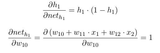
Multiply everything together, this is what we get:

This gives us the result of 0.01315. Following this method for the rest of the weights in theta1.

The reason why all the partial derivative are 0 except for w10 and w20 is because the input values are 0.

A vectorization way to manipulate the calculation above is

change_in_a2=theta2(:,2:end)'*((a3-y).*a3.*(1-a3));
delta1=change_in_a2.*a2(2:end).*(1-a2(2:end))*a1';

To update theta1 to reduce the error, the formula below is used with learning rate chosen at 0.5

new_theta1 = theta1 - 0.5*delta1; %update theta2 to reduce Error with learning rate is 0.5

Now all weights are updated to new values. Next, I perform the forward propagation again and get the output of 0.91611 which reduces the error to 0.41963 (it was 0.424529 before). Imagine performing this process over and over again will help to reduce the error close to 0. Therefore, the output value will get close to what we want.

I hope this helps you to understand backprop. I'm nowhere an expert at this; I'm just a student trying to learn from Prof. Andrew Ng's course. Thank you so much for making it until here. If you notice nay mistakes I made or simply unclear about anything, please contact me.

Here is the full code in Octave/Matlab which iterates for 10,000 times to reduce the error. The 'result' matrix at the end contains the iteration, error and output.

clc; clear;

%---------------Forward Propagation----------------------------
a1 = [1;0;0];                %first layer after adding the bias term 1
new_theta1 = [1 1 1; 1 1 1]; %weights of first layer
new_theta2 = [1 1 1];        %weights of second layer
y = [0];                     %expected output
learning_rate=0.5;           %initialize learning rate value

for i = 1:10000
  theta1  =new_theta1;
  theta2 = new_theta2;
z2 = theta1*a1;           %compute the net value of the hidden layer
a2 = 1./(1+exp(-z2));     %compute the activation units of hidden layer
a2 = [1;a2];              %adding bias term to the hidden layer
fprintf('\nThe second layer units are:\n');
fprintf('%f\n', a2);


z3 = theta2*a2;       %compute the net value of the output layer
a3 = 1./(1+exp(-z3)); %compute predictions
fprintf('\nThe third layer units are:\n');
fprintf('%f\n', a3);

%-------------Calculate Total Error-----------------------------------
error = (1/2)*(y-a3).^2;
fprintf('\nThe total error is: %f\n', error);

%-------------Backprop for the output layer---------------------------
delta3 = a3-y;
delta2 = delta3.*a3.*(1-a3)*a2';
new_theta2 = theta2 - 0.5*delta2;  %update theta2


%-------------Back propagation for the hidden layer-------------------
change_in_a2 = theta2(:,2:end)'*((a3-y).*a3.*(1-a3));
delta1 = change_in_a2.*a2(2:end).*(1-a2(2:end))*a1';
new_theta1 = theta1 - 0.5*delta1;                     %update theta1


%-------------Feed forward again to check results---------------------
z2 = new_theta1*a1;    %compute the net value of the hidden layer
a2 = 1./(1+exp(-z2));  %compute the activation units of hidden layer
a2 = [1;a2];           %adding bias term to the hidden layer

z3 = new_theta2*a2;    %compute the net value of the output layer
a3 = 1./(1+exp(-z3));  %compute output 

fprintf('\nThe new third layer units are: [%f]T\n', a3);
fprintf('The end of %f  time.\n', i);

result(i,:)=[i error a3]; %save all results in a matrix 
fprintf('==========\n');
endfor